
Load balancing and capacity planning: utilisation and Little’s law
Capacity planning answers one question: how much traffic can this system handle before it slows down or fails? A few formulas from queueing theory answer it surprisingly well.
Utilisation: the one number that predicts overload
A server with c parallel workers, each taking 1/μ seconds per request, can complete c·μ requests per second. Divide the arrival rate by that capacity and you get utilisation, ρ.
Below 1, the server keeps up on average. At or above 1, the queue grows without limit — the server will eventually run out of memory or start rejecting requests.
ρ = λ ÷ (c · μ)
Why latency explodes near 100%
Even below 100%, requests sometimes arrive in bunches and have to wait. The expected queue grows roughly like ρ ÷ (1 − ρ): modest at 50%, nine times larger at 90%, ninety-nine times larger at 99%.
That is why production systems target 60–70% utilisation and alert at 80%. The last few percent of capacity cost the most latency.
Little’s law
Little’s law connects three quantities for any stable system: the average number of requests inside it equals the arrival rate times the average time each spends inside.
It is the quickest way to size anything that holds a request: threads, connections, memory, serverless concurrency. 500 requests per second that each take 200 ms means about 100 in flight at any moment.
L = λ × W
Load balancing algorithms
A load balancer spreads requests across healthy targets. The algorithm matters most when targets differ in size or speed.
- Round robin: each target in turn. Simple and even when targets are identical.
- Least connections (least outstanding requests): send to the target with the fewest active requests. Adapts to slow or unequal targets.
- Weighted: target i receives a share wᵢ ÷ Σw of traffic. Useful for mixed instance sizes and gradual rollouts.
- Health checks: targets that fail checks receive no traffic. This is what turns redundancy into availability.
Autoscaling and its delays
Target-tracking autoscaling adds replicas when average CPU stays above a target: desired = ⌈current × utilisation ÷ target⌉. It works, but with two delays — the evaluation window and the replica start-up time.
During that gap, existing replicas absorb the extra load. Scaling earlier (a lower target), starting faster, or keeping more minimum replicas all shrink the gap.
Designing for failure
Every component eventually fails, so capacity has to include spare: N+1 instances, spread across availability zones, behind health-checked load balancers. When one fails, the rest must absorb its share — which only works if they were not already at 90%.
Slow dependencies are as dangerous as dead ones. Timeouts stop slowness spreading upstream; retries with exponential back-off and jitter recover transient failures without causing a retry storm.
Try it in the simulator
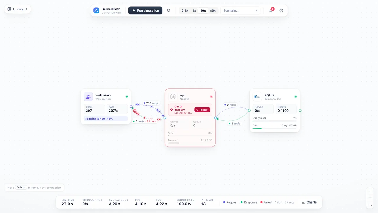 Small
Side project
One small server and an embedded database. Traffic ramps up until the single machine runs out of memory.
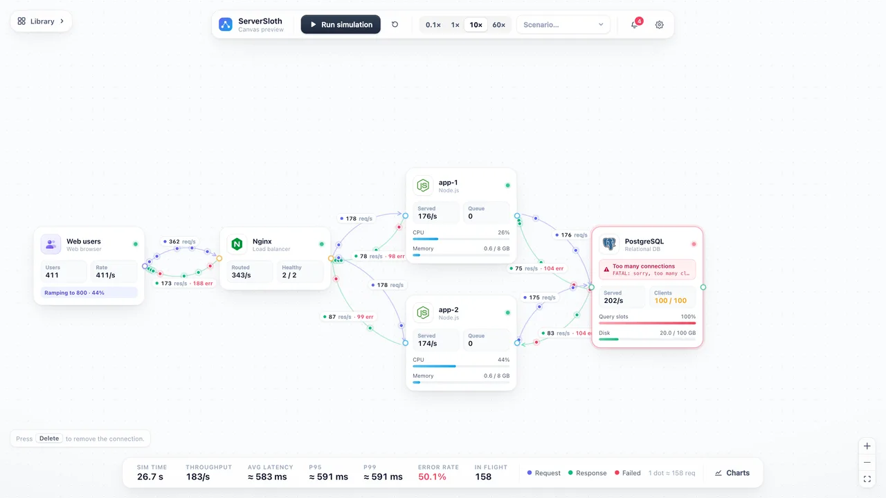 Startup
Small startup
Nginx in front of two app servers and one PostgreSQL. The app tier scales; the database becomes the bottleneck.
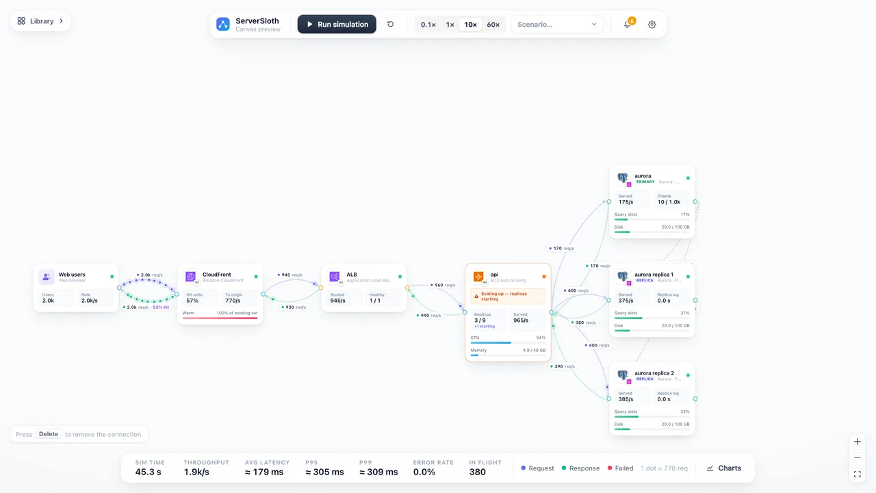 Scale-up
Read-heavy at scale
CloudFront → ALB → an auto-scaling group → Aurora with two read replicas. At 40 s the primary fails.
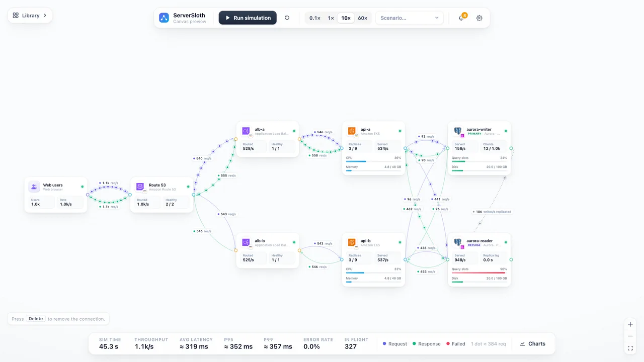 Global
Multi-region
Route 53 → two zones, each with an ALB and EKS → Aurora writer in zone A with a replica in zone B. Zone A fails at 40 s.
Failure modes in this guide
- Out of memory (OOM)
- When a node dies
- Availability zone outage
- CrashLoopBackOff
- Queue full (503)
- “Too many connections”
- Throttling and 429 Too Many Requests
- Serverless concurrency limits
- No healthy targets
- Timeouts and retries
- Fault injection and chaos engineering
- CPU saturation and queueing
- Serverless cold starts
- Autoscaling lag
- Max replicas reached
- Latency injection
- High load warnings